\( \newcommand\al{\alpha} \newcommand\be{\beta} \newcommand\de{\delta} \newcommand\De{\Delta} \newcommand\eps{\epsilon} \newcommand\ga{\gamma} \newcommand\Ga{\Gamma} \newcommand\ka{\kappa} \newcommand\la{\lambda} \newcommand\La{\Lambda} \newcommand\om{\omega} \newcommand\Om{\Omega} \newcommand\sg{\sigma} \newcommand\Sg{\Sigma} \renewcommand\th{\theta} %--- Latex uses \th for a Norse character \newcommand\Th{\Theta} \newcommand\vphi{\varphi} % % some calligraphy % \newcommand\cA{{\mathcal A}} \newcommand\cB{{\mathcal B}} \newcommand\cC{{\mathcal C}} \newcommand\cD{{\mathcal D}} \newcommand\cE{{\mathcal E}} \newcommand\cF{{\mathcal F}} \newcommand\cG{{\mathcal G}} \newcommand\cH{{\mathcal H}} \newcommand\cI{{\mathcal I}} \newcommand\cJ{{\mathcal J}} \newcommand\cK{{\mathcal K}} \newcommand\cL{{\mathcal L}} \newcommand\cM{{\mathcal M}} \newcommand\cN{{\mathcal N}} \newcommand\cO{{\mathcal O}} \newcommand\cP{{\mathcal P}} \newcommand\cQ{{\mathcal Q}} \newcommand\cR{{\mathcal R}} \newcommand\cS{{\mathcal S}} \newcommand\cT{{\mathcal T}} \newcommand\cU{{\mathcal U}} \newcommand\cV{{\mathcal V}} % % fields and rings (and a semigroup) % \newcommand\cx{{\mathbb C}}% complexes \newcommand\fld{{\mathbb F}} \newcommand\flde{{\mathbb E}} \newcommand\ints{{\mathbb Z}} \newcommand\nn{{\mathbb N}}%non-negative integers \newcommand\re{{\mathbb R}}%reals \newcommand\rats{{\mathbb Q}} % % the really useful stuff % \newcommand\comp[1]{{\mkern2mu\overline{\mkern-2mu#1}}} \newcommand\diff{\mathbin{\mkern-1.5mu\setminus\mkern-1.5mu}}% for \setminus \newcommand\res{\mathbin{\mkern-2.0mu\restriction\mkern-2.0mu}} \newcommand\sbs{\subseteq} \newcommand\sps{\supseteq} \newcommand\seq[3]{#1_{#2},\ldots,#1_{#3}} \DeclareMathOperator{\supp}{supp} \DeclareMathOperator{\im}{im} \DeclareMathOperator{\row}{row} \newcommand\pmat[1]{\begin{pmatrix} #1 \end{pmatrix}} \newcommand\cprod{\mathbin{\square}} \newcommand\gbin[2]{\genfrac{[}{]}{0pt}{}{#1}{#2}} % % matrix theory % \newcommand\ip[2]{\langle#1,#2\rangle} \newcommand\one{{\bf1}} \DeclareMathOperator{\rk}{rk} \DeclareMathOperator{\tr}{tr} \DeclareMathOperator{\col}{col} \newcommand\mat[3]{\mathrm{Mat}_{#1\times #2}(#3)} \newcommand\sm[3]{\sum_{#1=#2}^{#3}} % % some group theory % \newcommand\aut[1]{{\rm Aut}(#1)} \newcommand\fx[1]{{\rm fix}(#1)}% ch2 \newcommand\grp[1]{\langle #1\rangle} \newcommand\nrml{\vartriangleleft} \newcommand\nrmleq{\trianglelefteq} \DeclareMathOperator{\Sym}{Sym} \newcommand\sym[1]{\Sym(#1)} \DeclareMathOperator{\Alt}{Alt} \newcommand\alt[1]{\Alt(#1)} \)

Section5.1Factors of \(K_6\)

A 1-factor, is a subgraph which includes every vertex and is regular of degree \(1\). (Here we will use factor as an abbreviation for 1-factor; in some contexts people use the term factor to denote a spanning regular graph.) For \(K_6\) a 1-factor is a collection of \(3\) edges with no common vertices.

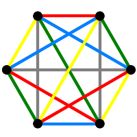
We build \(K_6\) first. We will work with sets of sets, so we convert the edges of \(K_6\) into two-element sets. Note that the vertices are integers, starting with zero. Also, we use the Sage constructor Set() rather than the Python version (set()), since these behave differently and we will have an easier time with the Sage version. Of course, \(K_6\) has \(6\) vertices and \({6\choose 2}=15\) edges. We will see these numbers repeatedly throughout this chapter.

We will give each of the \(15\) edges a name (an arbitrary lowercase letter) which will make some of our graphs a bit more tidy when displaying them. A Python dictionary (mapping) is a natural way to specify this.

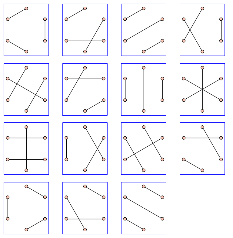
Since \(K_6\) includes every possible edge, a factor is partition of the vertex set into a set of three \(2\)-sets. We discover \(15\) factors.

We can easily visualize the \(15\) different factors by considering each factor as an edge-induced subgraph of \(K_6\). We build a list of these subgraphs and use a convenient utility in Sage to display them all simply and compactly. These \(15\) objects will be critical in what follows.

Figure5.1.1Fifteen one-factors of \(K_6\)

The edge-factor incidence graph is a remarkable graph. The Tutte \(8\)-cage is the cubic graph (i.e. regular of degree \(3\)) with girth \(8\) and having the fewest possible number of vertices. It therefore also qualifies as a Moore graph. Since it is distance-transitive, it is also distance-regular.

We use the set of edges and the set of factors as the vertex set of a graph. We join an edge to a factor if the edge is a component of the factor.

Since this graph is built into Sage, we can get a much more pleasing drawing from the embedding that is hard-coded. If we give our factors names (uppercase letters from the start of the alphabet), then we can relabel the vertices of a copy of the graph and use Sage's BipartiteGraph class to get another informative drawing.